SOURCE CODING AND LINE CODING Differences | MATCHED FILTER AND INTERSYMBOL INTERFERENCE (ISI)
DIFFERENCE BETWEEN SOURCE CODING AND LINE CODING , MATCHED FILTER AND INTERSYMBOL INTERFERENCE (ISI) :-
We can differentiate between source coding and line coding in the form of following points :
(i) We have already discussed various source coding techniques such as PCM, Delta modulation ADM etc.
(ii) Source coding technique are used in order to convert an analog signal to its digitally coded equivalent signal. The output of a source coder is a train of binary digits, i.e., 0s and ls.
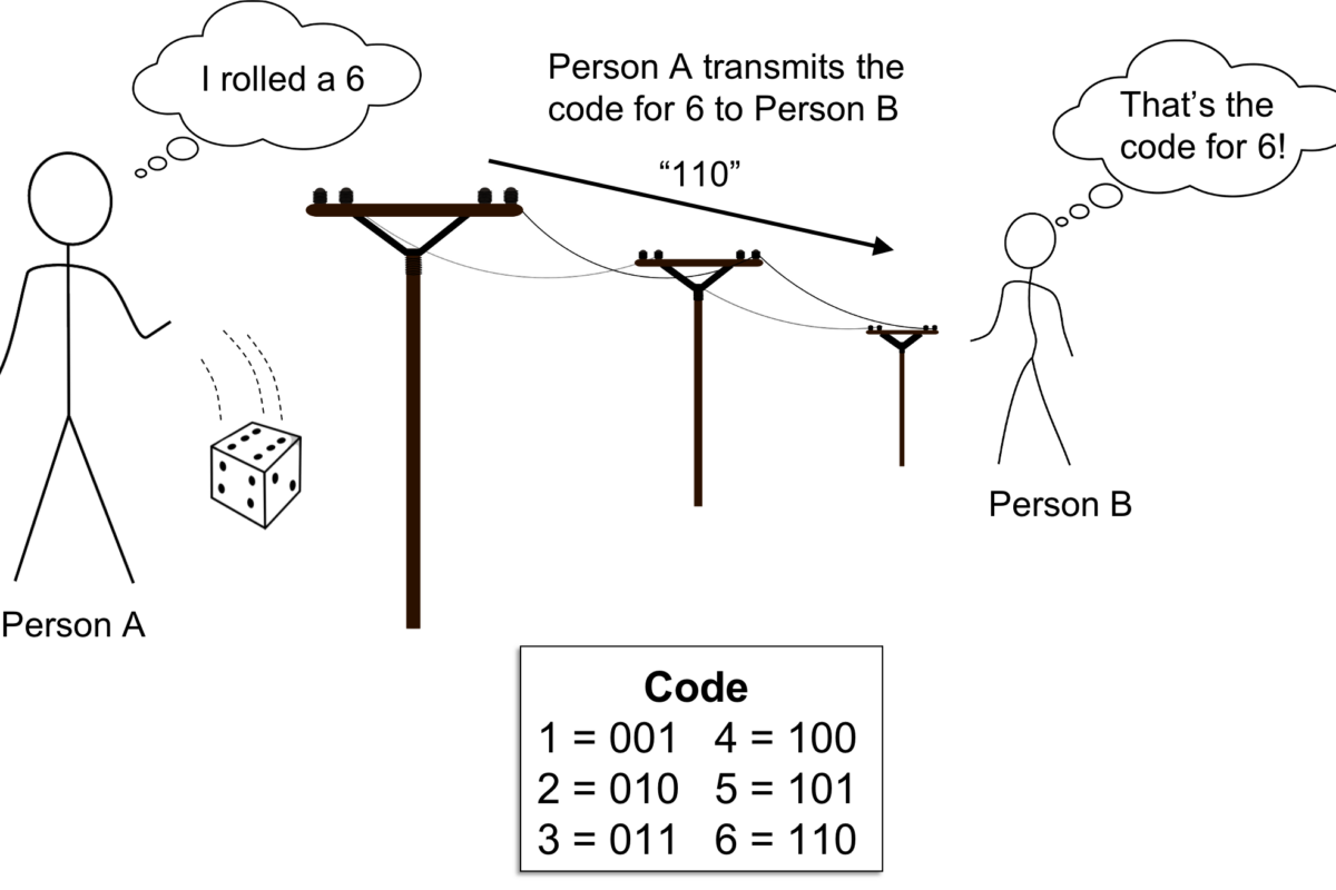
(iii) The line coding techniques convert the stream of binary digits into a format or code which is more suitable for transmission over a cable or any other medium.
(iv) This is because the data transmission must satisfy certain requirements such as synchronization, elimination of dc component, low cross talk etc.
(v) The line code formats should be such that the bandwidth requirements be as low as possible. Examples of line codes are RZ, NRZ, AMI, Manchester and other formats.
6.20 INTRODUCTION TO MATCHED FILTER AND INTERSYMBOL INTERFERENCE (ISI)
As discussed earlier, there are various techniques for converting an analog information-bearing signal into digital form. There is another way in which digital data can rise in practice that is the data may represent the output of a source of information which is inherently discrete in nature (e.g., a digital computer).
As a matter of fact, digital data have a broad spectrum with a significant low frequency content. Therefore, baseband transmission of digital data requires the use of a low-pass channel with a bandwidth large enough to accommodate the essential frequency content of the data stream. However, usually the channel is dispersive in that its frequency response deviates from that of an ideal low-pass filter (LPF).
The result of data transmission over such a channel is that each received pulse is affected somewhat by adjacent pulses and hence giving rise to a common form of interference called intersymbol interference (ISI).
Intersymbol interference (ISI) is a major source of bit errors in the reconstructed data stream at the receiver output. To correct for it, control has to be exercised over the pulse shape in the overall system.
Another source of bit error in a baseband data transmission system is the channel noise.
Basically, noise and ISI arise in the system simultaneously. However, to understand how they affect the performance of the system, let us first consider them separately. However, later on, we shall analyze their combined effects.
Now, let us describe a fundamental result in communication system which deals the detection of a pulse signal of known waveform that is immersed in additive white noise.
NOTE: In fact, the device for the optimum detection of such a pulse involves the use of a linear-time-invariant (LTI) filter which is known as a matched filter. The matched filter is so called because its impulse response is matched to the pulse signal.
6.21 INTEGRATE AND DUMP FILTER (i.e., RECEIVER)
Let us consider a very simple and basic detector circuit for the detection of digital signals. Figure 6.18 illustrates the circuit of such type of detector which is called an integrate and dump filter.
Here, the digital signal x(t) is distorted by white noise n(t) during the transmission over channel. This noisy signal [x(t) + n(t)] is applied to the input of integrate and dump filter. The capacitor is discharged fully at the beginning of the bit interval. This is achieved by temporarily closing switch S2 at the beginning of the bit interval. The integrator then integrates noisy input signal over one bit period. This integrated signal is shown as y(t) in the figure. For the square pulse input, the output of the integrator would be a triangular pulse as shown in figure 6.25.
DIAGRAM
FIGURE 6.25 Integrate and dump filter.
Figure 6.26(b) illustrates the waveform of y(t). At the end of bit period i.e., at t = T, the magnitude of y(l) attains its maximum amplitude. Hence, the value of y(t) is sampled at the end of bit period. It can be further proved that the signal to noise ratio is maximum at the end of bit period (i.e., at t = T). Depending upon the value of y(7), the decision is taken. The dump switch S2 is then closed momentarily to discharge the capacitor to receive the next bit. Therefore, the integrator integrates (i.e. generates output) which is independent of the value of previous bit. This reveals the fact that the detection in integrate and dump filter is unaffected by the values of previous bits. In figure 6.26(b), the output of integrator would decrease after t > T.
DIAGRAM
FIGURE 6.26 (a) Input pulse to the integrator (Here, we have assumed that the noise is absent). This pulse represents binary ‘1’. The width of pulse is “T” (b) Output of integrator. The initial output is zero. At t = T, the output of integrator is y(t) = AT.
6.21.1. Calculation of Signal to Noise Ratio for the Integrate and Dump Filter
We know that the output of the integrator may be written as,
EQUATION …(6.39)
Here, the integration is performed over one bit period i.e., from 0 to T. The noisy signal [x(t) + n(t)] is the input to the integrator. Equation (6.39) may be modified as
EQUATION …(6.40)
or y(t) = x0(t) + n0(t)
where x0(t) is the output signal voltage and n0(t) is the output noise voltage.
Now, let us consider output signal voltage which is
equation …(6.41)
Because the value of x(t) = A form 0 to T, the above equation can be written as,
EQUATION
Integrating, we get
x(t) =
or x0(t) = …(6.42)
Let the time constant be RC = .
Hence, equation (6.42) will become,
x0(t) = …(6.43)
The normalized signal power in standard resistance of 1 W would be,
Output signal power =
Putting the value of x0(t), we get
Output signal power = …(6.44)
Now, let us find the noise power. However, before doing so, we have to calculate the transfer function of the integrator. Recall that a network which performs integration operation has the transfer function equal to .*
Now, since a delay of t = T in time domain is equivalent to in frequency domain, therefore, the network performing integration over the period of T can be represented by the transfer function as under:
H(f) = …(6.45)
For = 2f and RC = , equation (6.45) takes theform
H(f) =
Separating, we get
EQUATION
Substituting the real and imaginary parts, we have
EQUATION
Then, the magnitude of above transfer function will become
EQUATION
Simplifying the last equation, we obtain,
…(4.46)
Now, the average power of the output noise signal n0(t) may be obtained by integrating its power density spectrum.
This means that
Power , EQUATION
For a standard 1 W resistance, the noise power would be .
Here, mean square value of noise signal is considered since it is a random signal. i.e.,
* In fact, this can be very, easily verified by taking the example of an RC circuit. The reason is that an RC low pass filter also basically performs integration operation.
** Using Euler’s identity = cos + j sin .
Noise power, …(6.47)
Again, we know that the input and output power spectral densities are related as,
Sno(f) = Sni(f) …(6.48)
where H(f) = transfer function of filter,
Sno(f) = power spectral density (psd) of output noise and
Sni(f) i = power spectral density (psd) of input noise.
Again, let us assume that white noise is present, therefore, the power spectral density (psd) of this noise would be,
Sni(f) = …(6.49)
Substituting this value in equation (6.48), we get
Sno(f) =
Substituting this value in equation (6.49), we have
EQUATION
Substituting the value of from equation (6.48) in above equation, we obtain
EQUATION …(6.50)
Now, let us substitute nf = x
so that dx = or
Further, since f =
therefore,
With all these substitutions, equation (6.51) becomes,
EQUATION
Rearranging above equation, we get
EQUATION
Now, let
so that du and limits will remain unchanged, therefore above equation will become.
EQUATION
Because, here the function is squared, the above equation can be written as,
EQUATION …(6.51)
This relation describes the noise power at the output. The signal to noise power ratio at output of integrator can be obtained as,
Signal power Signal to, =
Substituting the values of signal power from equation (6.44) and noise power from equation (6.51), we get
EQUATION
Hence, we conclude
Signal to Noise ratio of Integrate and Dump receiver:
= …(6.52)
This signal to noise ratio is also known as figure of Merit.
Few points about Signal to noise ratio:
(i) The result in equation (6.52) shows that signal to noise ratio improves in proportion to sampling period T. It is also increased as signal amplitude ‘A’ is increased.
(ii) Because noise has gaussian distribution and zero mean value at any time, therefore, the output of integrator also increases by a very small margin at the end of bit interval.
Figure 6.27 shows the waveform of x0(t) and n0(t) for the input signal x(t).
Figure 6.27 shows the waveforms of integrate and dump filter receiver for the rectangular pulses input.
It may observed that the output signal voltage reaches to the value of ± at the sampling instant. This is the maximum signal voltage. But the noise voltage n0(t) does not increase in same proportion. This is due to the fact that the noise has zero average value and Gaussian distribution.
DIAGRAM
FIGURE 6.27 (a) Input signal to the integrate and dump filter (b) Output signal of the integrate and dump filter (c) Output noise of the integrate and dump filter.
EXAMPLE 6.11. Show that for an integrate and dump filter receiver, the maximum signal to noise ratio is expressed as.
Given that the input signal x(t) is rectangular pulses of amplitudes ± A and duration T.
Solution : Receall that the energy of the signal x(t) is given by the relation
EQUATION
Given that x(t) is a rectangular pulse of amplitude ± A and duration, T1. Therefore, equation (i) can be written as
EQUATION ….(ii)
We know that the signal to noise ratio of integrate and dump filter receiver is given as,
….(iii)
Substituting, A2T = E from equation (ii) in equation (iii), we get
Since output is maximum at sampling instant, T, therefore, the above value is maximum i.e.,
Hence Proved
हिंदी माध्यम नोट्स
Class 6
Hindi social science science maths English
Class 7
Hindi social science science maths English
Class 8
Hindi social science science maths English
Class 9
Hindi social science science Maths English
Class 10
Hindi Social science science Maths English
Class 11
Hindi sociology physics physical education maths english economics geography History
chemistry business studies biology accountancy political science
Class 12
Hindi physics physical education maths english economics
chemistry business studies biology accountancy Political science History sociology
English medium Notes
Class 6
Hindi social science science maths English
Class 7
Hindi social science science maths English
Class 8
Hindi social science science maths English
Class 9
Hindi social science science Maths English
Class 10
Hindi Social science science Maths English
Class 11
Hindi physics physical education maths entrepreneurship english economics
chemistry business studies biology accountancy
Class 12
Hindi physics physical education maths entrepreneurship english economics